How to Perform Paired Samples T-Test with Julius
This article will provide a comprehensive review on how to properly use a paired samples t-test to assess means of two different groups in a ‘before and after’ research study.
Introduction
T-tests are statistical tests used to determine if the mean difference between two groups are statistically significant. They are often used in hypothesis testing when your dataset contains continuous variables.
There are different types of t-tests you can use depending on the nature of your data. Below is a brief overview of the common types of t-tests used:
1. Independent Samples t-test: Used when you have two independent groups that you would like to compare the means of. Your two groups must be sampled independently from one another. For example, you may use this test to compare the mean test scores from students between two different schools.
2. Paired Samples t-test (or Dependent t-test): Used when you compare the means of two related groups. It’s used when the same individual is measured under two different conditions at different points in time. For example, measuring blood pressure before treatment and then after treatment.
3. One-sample t-test: Used to test for significant differences between an unknown population mean and a known hypothesized value. For example, you can look at the average height of a group of high school students (unknown value) to the national average height (known hypothesized value).
The t-test we will be focusing on in this tutorial is the paired samples t-test. Before we assess the dataset, it is important to mention the various assumptions this test requires. These assumptions must be met for the results to be valid: the data to be normally distributed, paired observations must be independent, there must be homogeneity of variances, and finally the data should be measured in an interval or ratio scale.
Dataset Overview
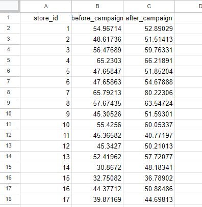
The dataset we will be using consists of monthly revenue figures (in thousands of dollars) for 100 stores. Revenue was recorded before the implementation of marketing campaigns and after it finished (approximately 4 weeks of advertisement). The purpose of this dataset is to evaluate the effectiveness of the campaign in increasing store revenue. A copy of the dataset can be found here. Below is a snapshot of the dataset.
Step-by-Step Walkthrough
Step 1: Load in Dataset
This walkthrough will be done using Python; however, you can also perform the analysis in Julius using R by switching the code runtime environment toggle in the top right of the chat interface.
To connect a dataset, you can either select the paperclip icon in the input bar to upload your data as a file, or you can also paste in a link to a publicly-shared Google Sheet. In this case, we are going to connect to a Google Sheet containing the diet and weight loss information.
Prompt: “Please preview the dataset from Google Sheets.”
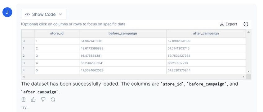
Above you can see that Julius has imported our dataset successfully. There are three columns: “store_id”, “before_campaign”, and “after_campaign”. This dataset has previously been examined for any missing or ‘null’ values, but please remember to do so with your own dataset before continuing with any analysis.
Step 2: Run Descriptive Statistics
Let’s prompt Julius to perform descriptive statistics on this dataset. We must specify the descriptives for each column to understand the distribution.
Prompt: “Can we perform descriptive statistics separately for the ‘before_campaign’ and ‘after_campaign’, please?”
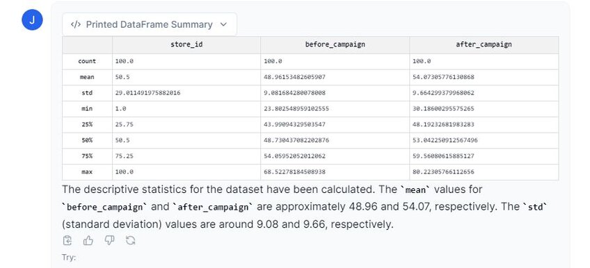
From the image above, we can already see some differences between the before and after campaign. For example, the mean for the before column is 48.96 (±SD = 9.08), whereas the after is 54.07 (±SD = 9.66). We can also see the differences in the minimum and maximum values, as well as the interquartile ranges vary.
Step 3: Testing Assumptions
Our next step is to test the various assumptions of a paired t-test. These assumptions are: the dataset assumes a normal distribution, variances are homogeneous, paired observations must be independent, and the dataset must be measured in interval or ratio scale. We can confirm the last two assumptions by examining our methodology – which we know from the setup that it passes both – but the normal distribution and homogeneity of variance must be tested.
Prompt 1: “Create a histogram and Q-Q plots on before_campaign and after_campaign columns. Then run a normality test to check for normality please.”
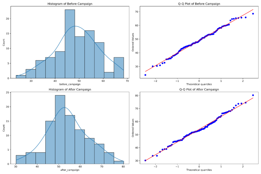
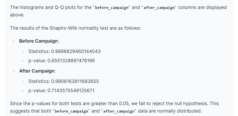
From the snapshots above, we can see that our dataset follows a normal distribution, which is required for the paired t-test analysis. We will now look at the homogeneity of variances.
Prompt 2: “Please perform a homogeneity of variances on both the ‘before_campaign’ and ‘after_campaign’.”
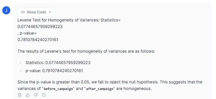
Above, we can see that our test statistic is 0.077, with a p-value of 0.78. This indicates that the variances are homogeneous between the groups, satisfying the assumption.
Step 4: Performing Paired T-Test
After checking the assumptions, we can now perform the paired t-test.
Prompt: “Please perform the paired t-test on the dataset.”
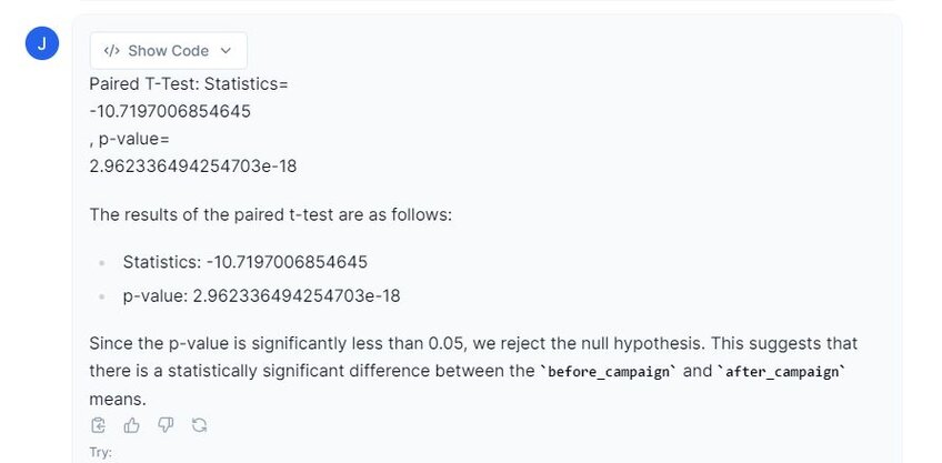
From the above results, we can conclude that there are statistically significant differences between revenue before the campaign and after the campaign. Thus, our results can be reported as follows: t(99) = -10.72, p ≤ 0.001.
In addition to this test, we can conduct an effect size test to understand the magnitude of difference between the before and after groups.
Prompt 2: “What is the effect size between the two groups?”

From the above image, we can see that Cohen’s d was approximately 1.07, indicating a large effect size. This suggests that these findings are not only statistically significant but also practically significant.
Now, adding in this information we can report these findings like this: t(99) = -10.72, p ≤ 0.001, d = 1.072.
Step 5: Visualizing the Difference
Our next step is to create a visualization that clearly shows the difference between the before_campaign and after_campaign revenue.
Prompt: “Please create a visualization that denotes statistical significance between the two groups.”
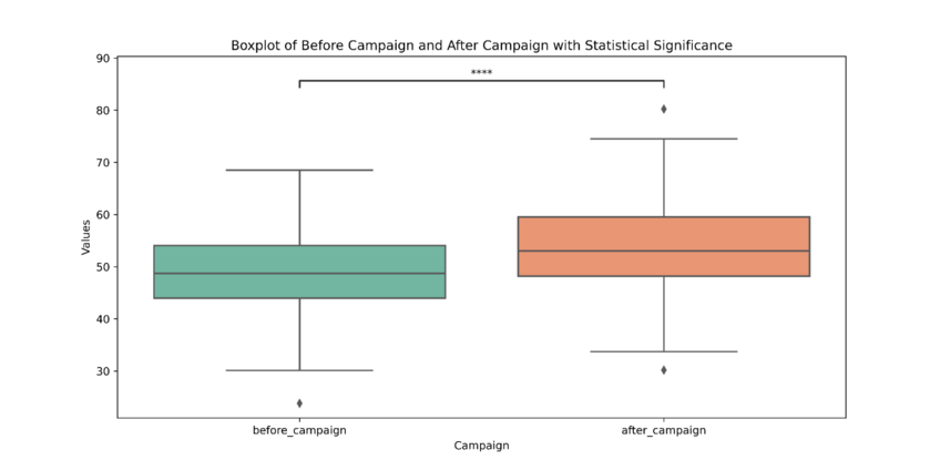
In the snapshot above, we can see that Julius has created a boxplot to show the statistically significant difference between before and after campaign. The four asterisks above the bracket indicate that the results were extremely significant.
Step 6: Reporting Results
Now that we have all this information, let’s summarize the main findings in a brief paragraph:
“A paired t-test was conducted to investigate if there was a difference in revenue before and after the campaign. Results showed a significant increase in revenue from before (48.96, ±SD = 9.08) and then after the campaign (54.07, ±SD = 9.66); t(99) = -10.72, p ≤ 0.001, d = 1.07. This indicates the campaign was successful in boosting sales."
Conclusion
In this use case, we learned the various types of t-tests and their applications, learned how to perform descriptive statistics on a marketing campaign, tested for the assumptions required for a paired t-test, and interpreted the results and effect size. Additionally, we discussed how to present our findings effectively and in a visually appealing manner. With the help of Julius, we can now confidently perform a paired t-test!
