

Combining two columns in Excel usually means picking one of 3 primary methods, depending on what you need to keep intact.
I've combined names, addresses, and phone number lists on sheets with thousands of rows, and the same handful of tricks covers almost every mess I've run into.
Here's how to pick the right one, plus how to keep dates and leading zeros intact without wrecking your original columns.
How to combine two columns in Excel: which method to use
Each method gets you to one combined column, but they fit different situations. Choose the one you need:
| 🔧 Method | 🎯 Best for | ⚡ Works in |
|---|---|---|
| Ampersand & | The quickest one-off join | Every Excel version (and Google Sheets) |
| CONCAT / TEXTJOIN | Clean delimiters, skipping blanks, joining many columns | Excel 2019, Microsoft 365, and Excel for the Web |
| Flash Fill | A no-formula cleanup you do once | Excel 2013 and later |
With these formulas, your original columns stay put. You're building the combined text in a new column, which makes it easy to check your work before you commit to anything.
Once you're happy with the result, you can lock it in and safely delete the source columns (I'll cover how further below).
💡 Tip: Power Query is a fourth option for very large or repeatable jobs, and I'll cover it after the three easy methods.
Method 1: the ampersand (&) operator
The ampersand (&) joins the contents of two or more cells into one. It's the method I reach for most because it works in every version of Excel and reads clearly once you've seen it once.
Here's how to use it:
Click the first empty cell in a new column, next to the rows you want to combine.
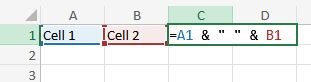
Type =A1 & " " & B1, swapping in your own cell references.
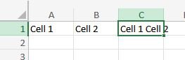
3. Press Enter. Excel shows the combined text, for example Cell 1 Cell 2
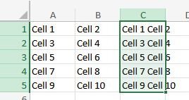
4. You don’t have to combine rows one at a time. If you want to combine multiple cells in a column, select that result cell, then drag the small square in its bottom-right corner (the fill handle) down the column, or double-click it to fill all the way to the last row of your data.
The " " in the middle is your delimiter, the character that sits between the two values. Swap it for whatever you need:
A space: =A1 & " " & B1
A comma and space: =A1 & ", " & B1
A dash: =A1 & "-" & B1
A line break (for address or name blocks): =A2 & CHAR(10) & B2, then turn on Wrap Text from the Home tab so the break shows.
💡Tip: The ampersand works exactly the same way in Google Sheets, so if you move between the two apps, this is the one syntax you don't have to relearn.
Method 2: the CONCAT and TEXTJOIN functions
If you're joining more than a couple of columns, or you want Excel to skip blank cells for you, the newer text functions are cleaner than stringing together a row of ampersands.
CONCAT joins values with no fuss:
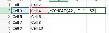
=CONCAT(A2, " ", B2) gives you the same result as the ampersand version.
TEXTJOIN is the one I lean on for anything bigger, because you only need to set the delimiter once:
=TEXTJOIN(" ", TRUE, A2, B2) joins the two cells with a space. The TRUE tells Excel to skip empty cells, so you don't end up with double spaces where a value is missing.
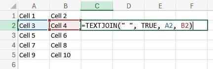
=TEXTJOIN(" ", TRUE, A2:B4) joins a whole range at once, which is how you combine a range of cells in a single formula.
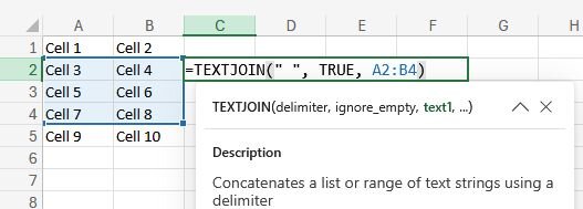
If you're on an older version of Excel, CONCATENATE is the legacy equivalent of CONCAT and still works.
💡Note: CONCAT and TEXTJOIN need Excel 2019, Microsoft 365, or Excel for the Web. On Excel 2016 or earlier they return a #NAME? error, which just means your version doesn't recognize the function. If you see that, use the ampersand or CONCATENATE instead.
Method 3: Flash Fill (no formula needed)
Flash Fill watches what you type and fills in the rest of the column once it spots the pattern. It's the fastest option when you'd rather not write a formula at all:
In a new column next to your data, type the combined result you want for the first row, for example Cell 1 Cell 2.
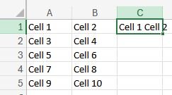
2. Start typing the second row. Excel usually previews the whole column in grey. 3. Press Enter to accept the preview. If nothing appears, put your cursor in the column or highlight the range you want to fill and press Ctrl/Cmd+E, or go to the Data tab and click Flash Fill.

If Flash Fill isn't kicking in automatically, you can turn it on under File > Options > Advanced > Automatically Flash Fill on Windows, or Excel > Preferences > Edit on Mac. Either way, Ctrl+E (Cmd+E on Mac) triggers it manually regardless of that setting.
I've run into a few limits you should know before you rely on this. The results are static text, so they won't update if the source data changes later, and the new column has to sit right next to the data it's reading from. I've also had Flash Fill misread messy or inconsistent data, so I scan the output before I trust it.
💡Tip: Reach for Flash Fill when you're cleaning up a list once. If the underlying data still changes, use one of the formula methods instead so the combined column updates with it. If you'd rather describe the join in plain English, you can use ChatGPT inside Excel to draft the formula for you.
Power Query for large or repeatable jobs
Power Query is the heavier option. I turn to it when I'm working with tens of thousands of rows, or when I know I'll run the same merge again next week.
Here's how it works:
Select your data, then go to Data > From Table/Range. This loads your data into Power Query.
Hold Ctrl and click the two column headers you want to join.
On the Add Column tab, click Merge Columns, pick a separator, and click OK.
Click Close & Load. This sends the combined result back to your worksheet.
The setup takes a bit longer than a formula, so I don't reach for it on a quick one-off task. But once it's built, the query re-runs every time you refresh it. I use this for monthly reports where the same 2 columns need combining every time, since it turns a repeat task into a single click.
💡 Note: Power Query has been in desktop Excel for Windows since 2016. On Mac, the full editor didn't arrive until 2023, and it's not supported at all in Excel 2016 or 2019 for Mac. On the web, it needs a Business or Enterprise Microsoft 365 plan for building new queries; a free or Personal plan won't have it.
How to combine columns with numbers, dates, or leading zeros
This is where a plain ampersand breaks, and it's easy to miss if you haven't hit it before.
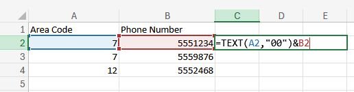
Excel stores dates as serial numbers behind the scenes, so =A7 & " " & B7 on a date can return something like 45844 instead of 07/06/2025. Numbers with leading zeros, like area codes or zip codes, lose the zero entirely.

The fix is the TEXT function, which forces a value to display in the format you choose before it gets joined:
Dates: =A7 & " " & TEXT(B7, "mm/dd/yyyy") keeps the date readable.
How to make the combined column permanent and delete the originals
Once your combined column looks right, you'll probably want to delete the two source columns to tidy up. If you try that while a formula is still in place, the result collapses into #REF! errors or blanks, because the formula is still pointing at cells you just removed.
The trick is to convert the formulas into plain text first:
Select your combined column and copy it with Ctrl+C.
Right-click the same cells and choose Paste Special > Values (or press Ctrl+Shift+V). This replaces the formulas with the actual text they produced.
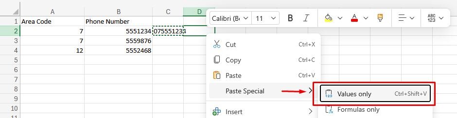
Now you can safely delete or hide the original columns. The combined column stands on its own.
💡Tip: Keep a copy of the original data on a separate sheet until you've confirmed the merge is correct. It's a cheap insurance policy against a bad delimiter or a misread pattern.
Skip Merge & Center for this
If you've reached for the Merge & Center button hoping it combines your data, that's the wrong tool, and it's worth saying why.
❌ Merge & Center merges cells but doesn’t merge their contents. It keeps only the value in the top-left cell and throws the rest away. It also can't update when your data changes, and merged cells break sorting, filtering, and formulas that reference them.

Use one of the formula methods or Flash Fill above instead. They combine the actual values and leave your data workable.
Common mistakes to avoid
I've made most of these mistakes myself at some point, and they trip people up more than the formulas do:
Forgetting a delimiter: =A2&B2 runs the two values together as JaneDoe. Add " " or another separator so the result is readable.
Combining into an existing column: Build the result in a new column instead, so you don't overwrite data you still need.
Deleting the source columns too soon: Convert the formula to values with Paste Special first, or the combined column breaks.
Trusting Flash Fill to update: It produces static text, so you'll need to re-run it or switch to a formula if the data changes.
Wrong number or date formatting: Wrap dates and zero-padded numbers in TEXT() so they read the way you expect.
If you find yourself combining the same columns every week, it's worth learning to record the steps as a macro, so Excel can repeat them for you in one click. A growing set of AI tools for Excel can also take on more of the combine-and-cleanup work for you.
Turn combined columns into answers, charts, and reports with Julius
Combining two columns in Excel gets your data clean, but cleanup isn't the finish line. Getting from that tidy sheet to an answer, chart, or report usually takes longer than the formula itself. Julius speeds up that next step.
Julius is an AI-powered data analysis tool, a sort of pocket data scientist. You ask questions in plain English and get back analysis with visuals already built, no formulas required.
Here's how Julius helps:
Data search: You can pull public data from the web or structured financial data through Julius's Financial Datasets integration, so you can start from a question instead of an upload.
Direct connections: Link databases like Postgres, Snowflake, and BigQuery, connect tools like Google Ads, or just upload your Excel or CSV file.
Built-in visualization: Ask a question and get back the analysis with charts already drawn, so you don't have to jump into another tool to build them.
One-click sharing: Turn your analysis into a PDF report you can send without reformatting.
Ready to skip the formulas and go straight to the answer? Try Julius for free today.
Frequently asked questions
How do I combine two columns in Excel without losing data?
Combine the columns into a new, empty column so you don't overwrite your originals. Once the combined column looks right, copy it and use Paste Special > Values to turn the formulas into plain text, and only then delete or hide the source columns. Keeping a backup copy of the original data on another sheet is a worthwhile extra step until you're sure.
What's the difference between the ampersand (&), CONCAT, and CONCATENATE?
All three join text and give you the same result. The ampersand is the fastest to type and works in every version of Excel plus Google Sheets, so it's the most portable. CONCAT is the modern function (Excel 2019 and Microsoft 365), and CONCATENATE is its older equivalent that still works in legacy versions for backward compatibility.
How do I combine two columns with a space, comma, or line break between them?
Put the character you want between the two cell references as a delimiter. Use " " for a space, ", " for a comma and space, or "-" for a dash, as in =A2 & ", " & B2. For a line break, use =A2 & CHAR(10) & B2 and turn on Wrap Text so the break displays.
How do I combine columns that contain numbers, dates, or leading zeros?
Wrap the number or date in the TEXT function so it keeps its formatting when joined. Use =A2 & " " & TEXT(B2, "mm/dd/yyyy") to keep a date readable, or =TEXT(A2, "00") & B2 to hold the leading zero on an area or zip code. Without TEXT, Excel shows dates as serial numbers and drops leading zeros.
How do I combine more than two columns at once?
Use TEXTJOIN with a range so you don’t have to list every cell. The formula =TEXTJOIN(" ", TRUE, A2:D2) joins columns A through D in one step, with a space between each value and blanks skipped. It's a cleaner way to merge three or more columns without a long chain of ampersands.