

I've had to compare data in two Excel sheets more times than I'd like to admit, and I've learned there isn't one "right" way to do it.
So for this one, I ran my usual four methods on the same two sheets to see how each performs.
Below, you'll find all 4 methods with exact steps and a quick way to pick which one fits your data.
How to compare data in two Excel sheets: pick your method
Every method here solves the same problem in a different way, so the right pick comes down to how your two sheets are built:
| 🧭 Method | ✅ Use this when | ⚡ Difficulty |
| View side by side | Small sheets, same layout, you just want a quick visual scan | Easy |
| Conditional formatting | Same layout and same row order, and you want differences highlighted in place | Easy |
| VLOOKUP or XLOOKUP | Rows are in a different order, or some records exist in one sheet but not the other | Medium |
| Spreadsheet Compare | Auditing two saved versions of a workbook (Windows only, enterprise/Pro Plus/LTSC editions) | Medium |
If your rows match position for position, conditional formatting or a side-by-side view works. If they don't, you need a lookup keyed on something unique, and that's what comes next.
Before you begin: set up a unique ID and your sample data
Once you know your rows can shift or go missing, you need a unique identifier in each sheet. A customer ID, an invoice number, or a SKU all work, anything that's one-of-a-kind per row. That's the anchor every lookup relies on.
Don't have a single unique column? You can build one. Pair two fields, like last name and order date, into one key, and it does the job. I cover the exact steps in this guide to combining columns.
To follow along, paste this into Sheet1 (cells A1:B4) and a slightly different copy into Sheet2. It's the sample I used to test every method below:
| Sheet1 ID | Sheet1 Amount | Sheet2 ID | Sheet2 Amount |
| 1001 | 500 | 1001 | 500 |
| 1002 | 620 | 1003 | 410 |
| 1003 | 410 | 1002 | 600 |
Notice that Sheet2 has the same IDs in a different order, and one amount changed. That's the realistic mess these methods have to survive.
Method 1: view two sheets side by side
You can compare two small sheets with matching layouts just by looking, without touching a single formula. This method works in Excel for Windows and in newer versions of Excel for Mac, but it isn't available in Excel for the web, so you'll need an up-to-date desktop app.
Excel's View Side by Side feature is built for comparing two separate open files. But if your two sheets are tabs inside the same workbook, you need one extra step first: opening a second window of that file, so Excel has two windows to arrange.
Here's how to set it up:
- Open your workbook and go to the View tab.
- Click New Window. Excel opens a second window of the same file.
- Click Arrange All, choose Vertical, check the box for Windows of Active Workbook (so Excel doesn't pull in every other file you have open), then click OK.
- Click your first sheet's tab in the first window, then your second sheet's tab in the second window.
- Turn on Synchronous Scrolling from the View tab so both panes scroll together.
Use method 1 when: You're on Excel desktop with two sheets under about 50 rows each, and you just need a quick gut-check before deciding whether the differences are worth a deeper look.
The honest limit: This method relies on your eyes catching every difference. It works fine on a few dozen rows, but scanning hundreds by hand is how mistakes slip through. Conditional formatting picks up where this one stops working, and that's next.
Method 2: highlight differences with conditional formatting
💡 Note: The screenshots below come from Excel for the web. Your version may vary slightly, depending on which platform and Excel version you're using.
Conditional formatting colors every cell that doesn't match between your two sheets, right where the data lives.
It's my default when both sheets share the same layout and row order, but there's a hard requirement: both sheets need to be tabs in the same workbook. If you've got two separate files, you'll need to copy one sheet into the other's workbook first, or use one of the lookup methods instead, which can pull data across files.
Here's how to set it up:
- Go to your first sheet and select the range you want to check. For our sample data, that's A2:B4.
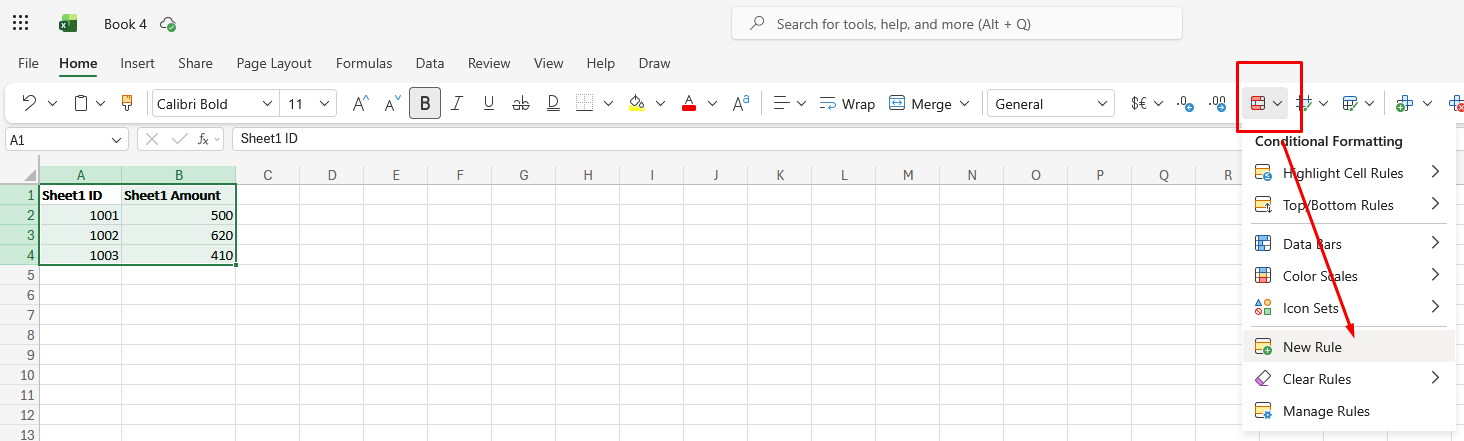
- On the Home tab, click Conditional Formatting, then New Rule.
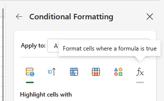
- Choose "Use a formula to determine which cells to format." (On Excel for Web, click the fx icon. Its tooltip reads "Format cells where a formula is true.")
- Enter a formula that compares each cell to its match on the other sheet:
=A2<>Sheet2!A2 - Click Format, choose a fill color, and click Done (or OK twice if you’re on desktop).
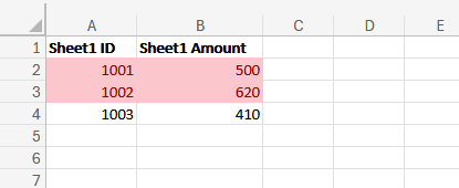
Every cell that doesn't match its twin on Sheet2 now lights up in your chosen color. From there, it's easy to turn those highlighted differences into a chart if you want to present the change visually.
💡 Tip: When you click a cell to build the formula, Excel adds dollar signs, like $A$2. Press F4 (or Fn+F4 on Mac) until the dollar signs disappear completely, usually three presses from where Excel first inserts them, so the reference reads A2 instead of $A$2.
Use method 2 when: Both sheets share the same layout and row order, and you want mismatches visible in place, with no extra columns needed.
The honest limit: Conditional formatting compares by position. Row 5 on one sheet gets checked against row 5 on the other, no matter what's actually in it. The moment your rows are sorted differently or a record goes missing, this method breaks down. For that, you need a lookup keyed on something unique, which is next.
Method 3: match rows with XLOOKUP or VLOOKUP
When rows sit in a different order, or some records only exist on one sheet, conditional formatting won't catch it since it only checks by position.
A lookup keyed on a unique ID finds the right row no matter where it sits. Our sample data is built for exactly this case, since Sheet2's rows are shuffled and one amount was changed.
The XLOOKUP version (Excel 365)
XLOOKUP is the cleaner option if you have it, mainly for its built-in fallback on missing values. In a new column on Sheet1, pull the matching amount from Sheet2:
=XLOOKUP(A2,Sheet2!$A:$A,Sheet2!$B:$B,"Missing")
If ID 1002 exists on Sheet2, you get its amount. If it doesn't, you get the word "Missing" in place of an error.
The VLOOKUP version (older Excel)
No XLOOKUP? VLOOKUP handles the same job. Wrap it in IFERROR so missing IDs read clearly:
=IFERROR(VLOOKUP(A2,Sheet2!$A:$B,2,FALSE),"Missing")
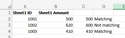
FALSE forces an exact match, and the absolute references (Sheet2!$A:$A and Sheet2!$A:$B) keep the range steady as you drag the formula down.
Flag what changed
Pulling the value across only gets you halfway there. Add one more column to show whether each row matches:
=IF(D2="Missing","ID missing",IF(D2<>B2,"Not matching","Matching"))
Filter that column, and you'll see only the mismatches and the missing IDs. This formula works the same whether you used XLOOKUP or VLOOKUP in the previous step, since it's just checking whatever value landed in column D.
Use method 3 when: Rows are out of order, records might be missing on either side, and you have, or can build, a unique ID column.
The honest limit: A lookup from Sheet1 only finds IDs that appear on Sheet1. Records that live only on Sheet2 never show up.
To catch both directions, build a helper column with =UNIQUE(VSTACK(Sheet1!A:A,Sheet2!A:A)) to get every ID from both sheets with duplicates removed. Then, run your lookup formulas against that column instead of just Sheet1's ID list.
Method 4: use Spreadsheet Compare
If you've got access, you can use Spreadsheet Compare to compare two saved versions of the same workbook. It also catches changes in any macros (the small automated scripts some workbooks use to run tasks behind the scenes).
Here's how to run it:
- Turn on the Inquire add-in first: File, Options, Add-Ins. At the bottom, switch the Manage dropdown to COM Add-ins and click Go. Check the box next to Inquire, then click OK.
- On the Inquire tab, click Compare Files.
- Choose the two files you want to compare, then click OK.
- Read the results in the two-pane grid. Excel color-codes each type of change, and the legend in the lower-left explains what each color means.
- Export the results to a new Excel file, or copy them into another program if you need a record.
Microsoft's own walkthrough covers the finer details of the results screen if you want to go deeper.
Use method 4 when: You're auditing versions of the same workbook, you need a change trail for something like an audit, and you're on an eligible edition of Excel.
The honest limit: Spreadsheet Compare only runs on Excel for Windows, and only on Microsoft 365 Apps for enterprise, Office Professional Plus (2013, 2016, or 2019), or Office LTSC 2021. Standard Microsoft 365 Business and Personal plans don't include it, and neither does Mac or Excel for the web.
Finding matches, missing rows, and duplicates
💡 Note: These formulas assume Sheet2 is a tab in the same workbook as Sheet1. If your two sheets are separate files, you can still reference them, but you'll need the full file path in your formula instead of just the sheet name.
Sometimes you only want an answer to one specific question. Here are the three that come up most:
Find matching rows
To confirm which IDs show up in both sheets, count how many times each one appears on the other sheet:
=COUNTIF(Sheet2!A:A,A2)>0
TRUE means the ID exists in Sheet2. FALSE means it doesn't.
Find missing rows
To spot records that live in one sheet but not the other, check whether a match exists at all:
=ISNA(MATCH(A2,Sheet2!A:A,0))
TRUE means the value from Sheet1 is missing on Sheet2. Run the same formula in reverse, Sheet2 against Sheet1, to catch what's missing the other way.
Find duplicates
To find IDs that repeat within a single sheet, check how many times each one shows up in that same column:
=COUNTIF(A:A,A2)>1
TRUE means that ID appears more than once on this sheet, worth cleaning up before you compare anything else. Run the same check on Sheet2 to catch duplicates there too.
You can also select the range, then go to Home, Conditional Formatting, Highlight Cells Rules, Duplicate Values, to color every repeat simultaneously.
Why your lookup says "no match"
You've written a clean VLOOKUP, the IDs clearly match, and Excel still returns "Missing."
I've run into this more than once, and the most common cause is numbers stored as text. If your IDs sit left-aligned in the cell, Excel is reading them as text (right-aligned means numbers). A text "1002" will never match a numeric 1002.
Fix it with Data, Text to Columns, or add a helper column with the VALUE function and paste those results back over the original column as values.
A few others worth checking:
- Absolute references: If you dragged a formula down and the lookup range shifted with it, lock it in place with dollar signs, like
$A$2:$B$28. - Trailing spaces: An invisible space after "1002 " breaks the match. Wrap your lookup value in TRIM to clean it.
- VLOOKUP can't look left: It only searches to the right of the key column. If your ID sits to the right of the value you want, use INDEX and MATCH, or XLOOKUP, which searches in either direction.
For heavier cleanup before you even start comparing, this guide to Excel data analysis covers the prep that makes lookups behave.
Want a quicker way to compare data? Try Julius
The four methods above work well when you compare data in two Excel sheets once, but they get harder to manage as your sheets grow, or the comparison becomes a regular part of your job.
Julius is an AI-powered data analysis platform that can search for public data or connect directly to your existing data sources, then return charts, insights, and reports from a single prompt.
Here's how Julius helps:
- Ask in plain English: Upload or connect both sheets and ask what changed between them. No VLOOKUP formula or conditional formatting rule required.
- Reconcile and explain: Julius matches records across both sheets and can explain what's driving the differences beyond which cells changed.
- Visualize the differences: Turn the mismatches into a chart in one step, so the change is easy to see at a glance.
- Clean up messy data first: Fix issues like numbers stored as text or extra trailing spaces before you compare without writing a TRIM or VALUE formula yourself.
- Learns your data as you go: Julius includes a Learning Sub Agent that learns the structure and relationships in your connected data as you use it, which can help results get more accurate with each query.
Ready to skip the formulas and ask what changed instead? Try Julius for free today.
Frequently asked questions
How do I compare two Excel sheets for differences?
You compare two Excel sheets by matching them either by position or by a unique key. If the layouts and row order match, use conditional formatting or a side-by-side view to spot differences. If the rows are out of order or records are missing, use VLOOKUP or XLOOKUP keyed on a unique ID.
How do I use VLOOKUP to compare two sheets?
VLOOKUP compares two sheets by pulling a matching value from the second sheet into the first. Write =IFERROR(VLOOKUP(A2,Sheet2!$A:$B,2,FALSE),"Missing") next to your data, then add an IF formula to flag whether each returned value matches or is missing.
Can Excel compare two sheets automatically?
Yes, Excel can compare two sheets automatically. Conditional formatting highlights differing cells live as data changes. The Spreadsheet Compare tool goes further, comparing two entire workbook versions and color-coding every change, though it's limited to Windows with Microsoft 365 Apps for enterprise, Office Professional Plus, or Office LTSC.
How do I find data that's in one sheet but not the other?
You find records unique to one sheet with a lookup that flags misses. Use =XLOOKUP(A2,Sheet2!A:A,Sheet2!B:B,"Missing") or =ISNA(MATCH(A2,Sheet2!A:A,0)), then run the same check in reverse to catch records missing from the other direction too.
Why isn't my VLOOKUP matching identical-looking values?
Your VLOOKUP usually fails because the values aren't as identical as they look. The most common cause is numbers stored as text (they sit left-aligned in the cell, where real numbers sit right-aligned), followed by trailing spaces and references that shifted when you dragged the formula. Fix them with VALUE, TRIM, and absolute references.